Quickstart¶

tsfeast¶

build

A collection of Scikit-Learn compatible time series transformers and tools.

Installation¶

Create a virtual environment and install:

From PyPi¶

pip install tsfeast

From this repo¶

pip install git+https://github.com/chris-santiago/tsfeast.git

Use¶

Preliminaries¶

This example shows both the use of individual transformers and the TimeSeriesFeatures convenience class that wraps multiple transformers. Both methods are compatible with Scikit-Learn Pipeline objects.

import warnings
warnings.filterwarnings("ignore")  # ignore pandas concat warnings from statsmodels

import pandas as pd
import numpy as np
import matplotlib.pyplot as plt

from sklearn.linear_model import LinearRegression, Lasso, PoissonRegressor
from sklearn.pipeline import Pipeline
from sklearn.feature_selection import SelectKBest
from sklearn.metrics import mean_squared_error, mean_absolute_percentage_error, mean_absolute_error
from sklearn.preprocessing import MinMaxScaler, StandardScaler
from statsmodels.tsa.arima_process import arma_generate_sample
from steps.forward import ForwardSelector

from tsfeast.transformers import DateTimeFeatures, InteractionFeatures, LagFeatures
from tsfeast.tsfeatures import TimeSeriesFeatures
from tsfeast.funcs import get_datetime_features
from tsfeast.utils import plot_diag
from tsfeast.models import ARMARegressor

def make_dummy_data(n=200):
    n_lags = 2
    coefs = {'ar': [1, -0.85], 'ma': [1, 0], 'trend': 3.2, 'bdays_in_month': 231, 'marketing': 0.0026}
    rng = np.random.default_rng(seed=42)
    
    sales = pd.DataFrame({
        'date': pd.date_range(end='2020-08-31', periods=n, freq='M'),
        'sales_base': rng.poisson(200, n),
        'sales_ar': arma_generate_sample(ar=coefs['ar'], ma=coefs['ma'], nsample=n, scale=100),
        'sales_trend': [x * coefs['trend'] + rng.poisson(300) for x in range(1, n+1)],
    })
    
    sales = sales.join(get_datetime_features(sales['date'])[['bdays_in_month', 'quarter']])
    sales['sales_per_day'] = sales['bdays_in_month'] * coefs['bdays_in_month'] + rng.poisson(100, n)
    
    sales['mkt_base'] = rng.normal(1e6, 1e4, n)
    sales['mkt_trend'] = np.array([x * 5e3 for x in range(1, n+1)]) + rng.poisson(100)
    sales['mkt_season'] = np.where(sales['quarter'] == 3, sales['mkt_base'] * .35, 0)
    sales['mkt_total'] = sales.loc[:, 'mkt_base': 'mkt_season'].sum(1) + rng.poisson(100, n)
    sales['sales_mkting'] = sales['mkt_total'].shift(n_lags) * coefs['marketing']
    
    final = pd.DataFrame({
        'y': sales[['sales_base', 'sales_ar', 'sales_trend', 'sales_per_day', 'sales_mkting']].sum(1).astype(int),
        'date': sales['date'],
        'marketing': sales['mkt_total'],
        'x2': rng.random(n),
        'x3': rng.normal(loc=320, scale=4, size=n)
    })
    return sales.iloc[2:, :], final.iloc[2:, :]

def get_results(estimator, x_train, x_test, y_train, y_test):
    return pd.DataFrame(
        {
            'training': [
                mean_absolute_error(y_train, estimator.predict(x_train)), 
                mean_absolute_percentage_error(y_train, estimator.predict(x_train))
            ],
            'testing':  [
                mean_absolute_error(y_test, estimator.predict(x_test)), 
                mean_absolute_percentage_error(y_test, estimator.predict(x_test))
            ],
        },
        index = ['MAE', 'MAPE']
    )

Example Data¶

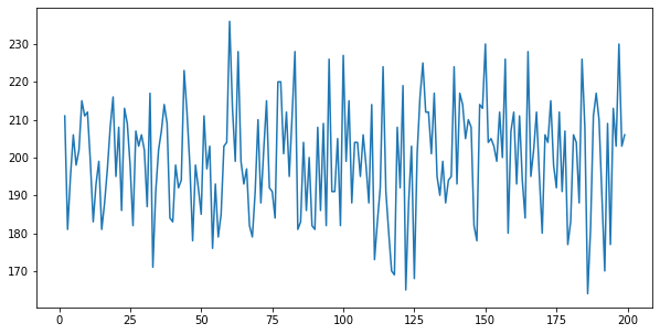
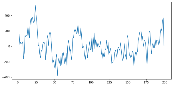
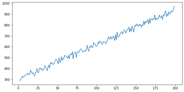
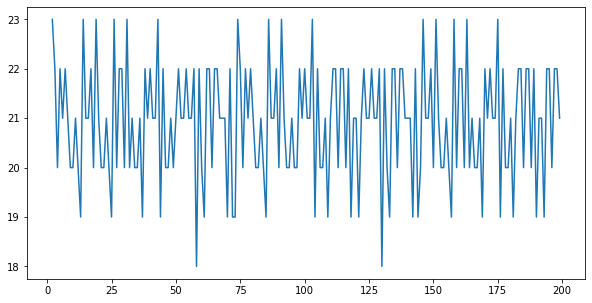
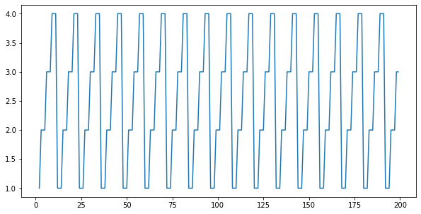
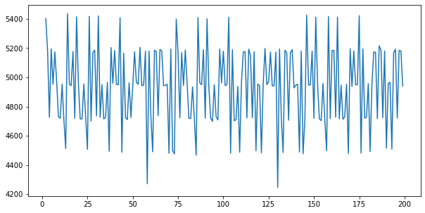
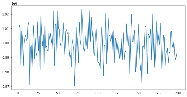
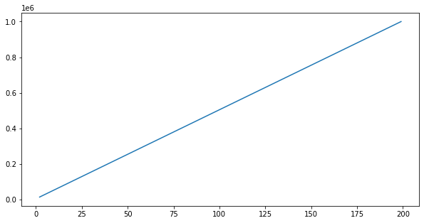
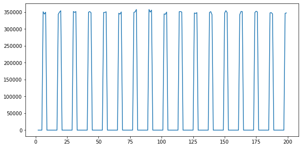
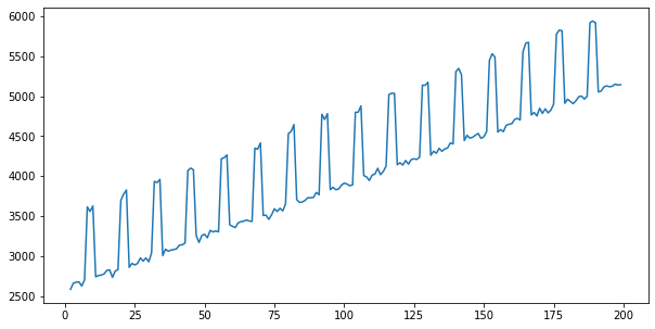
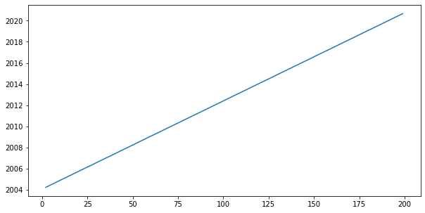
The dummy dataset in this example includes trend, seasonal, autoregressive and other factor components. Below, we visualize the individual components (comps) and features of the dummy dataset data.

comps, data = make_dummy_data()

Sales Components¶

comps.head()

	date	sales_base	sales_ar	sales_trend	bdays_in_month	quarter	sales_per_day	mkt_base	mkt_trend	mkt_season	mkt_total	sales_mkting
2	2004-03-31	211	153.620257	285.6	23	1	5402	1.012456e+06	15128.0	0.000000	1.027692e+06	2584.285914
3	2004-04-30	181	18.958345	300.8	22	2	5180	1.009596e+06	20128.0	0.000000	1.029835e+06	2661.116408
4	2004-05-31	195	54.420246	312.0	20	2	4726	9.848525e+05	25128.0	0.000000	1.010071e+06	2672.000109
5	2004-06-30	206	31.100042	326.2	22	2	5195	1.008291e+06	30128.0	0.000000	1.038529e+06	2677.570754
6	2004-07-31	198	34.283905	317.4	21	3	4952	1.004049e+06	35128.0	351416.992807	1.390691e+06	2626.185776

for col in comps.columns:
    print(f'Column: {col}')
    plt.figure(figsize=(10, 5))
    plt.plot(comps[col])
    plt.show()

Column: date

png

Column: sales_base

png

Column: sales_ar

png

Column: sales_trend

png

Column: bdays_in_month

png

Column: quarter

png

Column: sales_per_day

png

Column: mkt_base

png

Column: mkt_trend

png

Column: mkt_season

png

Column: mkt_total

png

Column: sales_mkting

png

Dummy Dataset¶

data.head()

	y	date	marketing	x2	x3
2	8636	2004-03-31	1.027692e+06	0.716752	316.389974
3	8341	2004-04-30	1.029835e+06	0.466509	318.780107
4	7959	2004-05-31	1.010071e+06	0.361299	324.917503
5	8435	2004-06-30	1.038529e+06	0.852623	316.776026
6	8127	2004-07-31	1.390691e+06	0.571951	314.425310

for col in data.columns:
    print(f'Column: {col}')
    plt.figure(figsize=(10, 5))
    plt.plot(data[col])
    plt.show()

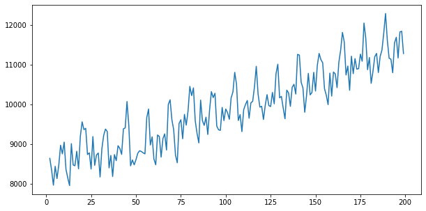
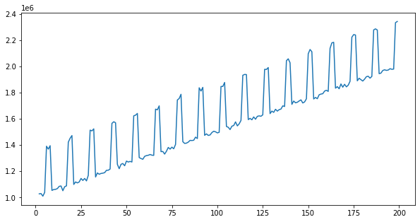
Column: y

png

Column: date

png

Column: marketing

png

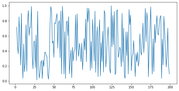
Column: x2

png

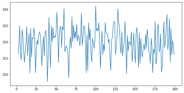
Column: x3

png

X = data.iloc[:, 1:]
y = data.iloc[:, 0]
x_train, x_test = X.iloc[:-40, :], X.iloc[-40:, :]
y_train, y_test = y.iloc[:-40], y.iloc[-40:]

Individual Transformers¶

tsfeast provides individual time series transformers that can be used by themselves or within Scikit-Learn Pipeline objects:

Transformer	Parameters	Description
`OriginalFeatures`	None	Passes original features through pipeline.
`Scaler`	None	Wraps Scikit-Learn `StandardScaler` to maintain DataFrame columns.
`DateTimeFeatures`	date_col: `str`, dt_format: `str`, freq: `str`	Generates datetime features from a given date column.
`LaggedFeatures`	n_lags: `int`, fillna: `bool`	Generate lag features.
`RollingFeatures`	window_lengths: `List[int]`, fillna: `bool`	Generate rolling features (mean, std, min, max) for each specified window length.
`EwmaFeatures`	window_lengths: `List[int]`, fillna: `bool`	Generate exponentially-weighted moving average for each specified window length.
`ChangeFeatures`	period_lengths: `List[int]`, fillna: `bool`	Generate percent change for all features for each specified period length.
`DifferenceFeatures`	n_diffs: `int`, fillna: `bool`	Generate `n` differences for all features.
`PolyFeatures`	degree: `int`	Generate polynomial features.
`InteractionFeatures`	None	Wraps Scikit-Learn `PolynomialFeatures` to generate interaction features and maintain DataFrame columns.

Notes on Pipeline Use¶

Behavior of Scikit-Learn Pipeline objects is appropriate and intended for independent data observations, but not necessarily appropriate for the temporal dependencies inherent in time series.

Scikit-Learn pipelines only call the .transform() method during the .predict() method, which is appropriate to prevent data leakage in predictions. However, most of the transformers in this package take a set of features and generate new features; there’s no inherent method to transform some time series features given a fitted estimator.

For time series lags, changes, etc., we have access to past data for feature generation without risk of data leakage; certain features (e.g. lags) require this to avoid NaNs or zeros. This behavior is appropriate for time series transformations, only.

Generate DateTime Features¶

dt = DateTimeFeatures(date_col='date')
dt.fit_transform(X, y)

	year	quarter	month	days_in_month	bdays_in_month	leap_year
2	2004	1	3	31	23	1
3	2004	2	4	30	22	1
4	2004	2	5	31	20	1
5	2004	2	6	30	22	1
6	2004	3	7	31	21	1
...	...	...	...	...	...	...
195	2020	2	4	30	22	1
196	2020	2	5	31	20	1
197	2020	2	6	30	22	1
198	2020	3	7	31	22	1
199	2020	3	8	31	21	1

198 rows × 6 columns

Generate Interaction Features¶

feat = LagFeatures(n_lags=4)
feat.fit_transform(X.iloc[:, 1:], y)  # skipping date column

	marketing_lag_1	x2_lag_1	x3_lag_1	marketing_lag_2	x2_lag_2	x3_lag_2	marketing_lag_3	x2_lag_3	x3_lag_3	marketing_lag_4	x2_lag_4	x3_lag_4
2	0.000000e+00	0.000000	0.000000	0.000000e+00	0.000000	0.000000	0.000000e+00	0.000000	0.000000	0.000000e+00	0.000000	0.000000
3	1.027692e+06	0.716752	316.389974	0.000000e+00	0.000000	0.000000	0.000000e+00	0.000000	0.000000	0.000000e+00	0.000000	0.000000
4	1.029835e+06	0.466509	318.780107	1.027692e+06	0.716752	316.389974	0.000000e+00	0.000000	0.000000	0.000000e+00	0.000000	0.000000
5	1.010071e+06	0.361299	324.917503	1.029835e+06	0.466509	318.780107	1.027692e+06	0.716752	316.389974	0.000000e+00	0.000000	0.000000
6	1.038529e+06	0.852623	316.776026	1.010071e+06	0.361299	324.917503	1.029835e+06	0.466509	318.780107	1.027692e+06	0.716752	316.389974
...	...	...	...	...	...	...	...	...	...	...	...	...
195	1.971301e+06	0.420222	313.911203	1.968782e+06	0.648398	327.288221	1.973312e+06	0.860346	319.932653	1.967943e+06	0.216269	317.692606
196	1.981624e+06	0.188104	324.110324	1.971301e+06	0.420222	313.911203	1.968782e+06	0.648398	327.288221	1.973312e+06	0.860346	319.932653
197	1.977056e+06	0.339024	315.926738	1.981624e+06	0.188104	324.110324	1.971301e+06	0.420222	313.911203	1.968782e+06	0.648398	327.288221
198	1.978757e+06	0.703778	320.409889	1.977056e+06	0.339024	315.926738	1.981624e+06	0.188104	324.110324	1.971301e+06	0.420222	313.911203
199	2.332540e+06	0.204360	319.029524	1.978757e+06	0.703778	320.409889	1.977056e+06	0.339024	315.926738	1.981624e+06	0.188104	324.110324

198 rows × 12 columns

TimeSeriesFeatures Class¶

tsfeast also includes a TimeSeriesFeatures class that generates multiple time series features in one transformer. The only required parameter is the column of datetimes; the optional parameters control what additional transformers are included.

Parameter	Type	Description
datetime	str	Column that holds datetime information
trend	str	Trend to include, options are {‘n’: no trend, ‘c’: constant only, ‘t’: linear trend, ‘ct’: constant and linear trend, ‘ctt’: constant, linear and quadratric trend}; defaults to no trend
lags	int	Number of lags to include (optional).
rolling	List[int]	Number of rolling windows to include (optional).
ewma	List[int]	Number of ewma windows to include (optional).
pct_chg	List[int]	Periods to use for percent change features (optional).
diffs	int	Number of differences to include (optional).
polynomial	int	Polynomial(s) to include (optional).
interactions	bool	Whether to include interactions of original featutes; deault True.
fillna	bool	Whether to fill NaN values with zero; default True.

feat = TimeSeriesFeatures(
    datetime='date',
    trend='t',
    lags=4,
    interactions=False,
    polynomial=3
)
features = feat.fit_transform(X, y)

features.head()

	trend	original__marketing	original__x2	original__x3	datetime__year	datetime__quarter	datetime__month	datetime__days_in_month	datetime__bdays_in_month	datetime__leap_year	...	features__lags__x3_lag_3	features__lags__marketing_lag_4	features__lags__x2_lag_4	features__lags__x3_lag_4	features__polynomial__marketing^2	features__polynomial__x2^2	features__polynomial__x3^2	features__polynomial__marketing^3	features__polynomial__x2^3	features__polynomial__x3^3
0	1.0	1.027692e+06	0.716752	316.389974	2004.0	1.0	3.0	31.0	23.0	1.0	...	0.000000	0.000000e+00	0.000000	0.000000	1.056152e+12	0.513733	100102.615631	1.085399e+18	0.368219	3.167146e+07
1	2.0	1.029835e+06	0.466509	318.780107	2004.0	2.0	4.0	30.0	22.0	1.0	...	0.000000	0.000000e+00	0.000000	0.000000	1.060560e+12	0.217631	101620.756699	1.092202e+18	0.101527	3.239468e+07
2	3.0	1.010071e+06	0.361299	324.917503	2004.0	2.0	5.0	31.0	20.0	1.0	...	0.000000	0.000000e+00	0.000000	0.000000	1.020244e+12	0.130537	105571.383672	1.030520e+18	0.047163	3.430199e+07
3	4.0	1.038529e+06	0.852623	316.776026	2004.0	2.0	6.0	30.0	22.0	1.0	...	316.389974	0.000000e+00	0.000000	0.000000	1.078543e+12	0.726966	100347.050373	1.120098e+18	0.619827	3.178754e+07
4	5.0	1.390691e+06	0.571951	314.425310	2004.0	3.0	7.0	31.0	21.0	1.0	...	318.780107	1.027692e+06	0.716752	316.389974	1.934020e+12	0.327128	98863.275608	2.689624e+18	0.187101	3.108512e+07

5 rows × 28 columns

[x for x in features.columns]

['trend',
 'original__marketing',
 'original__x2',
 'original__x3',
 'datetime__year',
 'datetime__quarter',
 'datetime__month',
 'datetime__days_in_month',
 'datetime__bdays_in_month',
 'datetime__leap_year',
 'features__lags__marketing_lag_1',
 'features__lags__x2_lag_1',
 'features__lags__x3_lag_1',
 'features__lags__marketing_lag_2',
 'features__lags__x2_lag_2',
 'features__lags__x3_lag_2',
 'features__lags__marketing_lag_3',
 'features__lags__x2_lag_3',
 'features__lags__x3_lag_3',
 'features__lags__marketing_lag_4',
 'features__lags__x2_lag_4',
 'features__lags__x3_lag_4',
 'features__polynomial__marketing^2',
 'features__polynomial__x2^2',
 'features__polynomial__x3^2',
 'features__polynomial__marketing^3',
 'features__polynomial__x2^3',
 'features__polynomial__x3^3']

Pipeline Example¶

The TimeSeriesFeatures class can be used as a feature generation step within a Scikit-Learn Pipeline. Given the temporal nature of the data and models, this may not be appropriate for all use cases– though the class remains fully compatible with Pipeline objects.

We’ll instantiate a TimeSeriesFeatures object with a linear trend, four lags and no interactions. Our pipeline will include feature generation, feature scaling and feature selection steps, before modeling with ordinary least squares.

Note: the ForwardSelector class is available in the step-select package (https://pypi.org/project/step-select/).

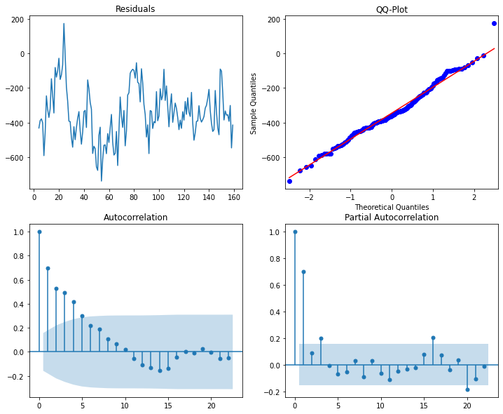
The pipeline creates a total of 22 features, before selecting only four to use in the final model. Note that 3 of the 4 final features corresponed with features from our “true model” that created the dummy dataset (‘trend’, ‘datetime__bdays_in_month’ and ‘marketing_lag_2’).

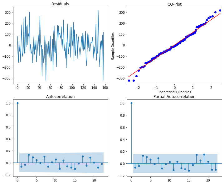
Regression diagnostic plots show evidence of slightly non-normal residuals and (1) autoregressive term (again, as specified in the “true model”). We’ll address the autoregressive term in the next example.

feat = TimeSeriesFeatures(
    datetime='date',
    trend='t',
    lags=4,
    interactions=False
)

pl = Pipeline([
    ('feature_extraction', feat),
    ('scaler', StandardScaler()),
    ('feature_selection', ForwardSelector(metric='bic')),
    ('regression', LinearRegression())
])

pl.fit(x_train, y_train)

Pipeline(steps=[('feature_extraction',
                 TimeSeriesFeatures(datetime='date', interactions=False, lags=4,
                                    trend='t')),
                ('scaler', StandardScaler()),
                ('feature_selection', ForwardSelector(metric='bic')),
                ('regression', LinearRegression())])

pl.named_steps.feature_extraction.output_features_

	trend	original__marketing	original__x2	original__x3	datetime__year	datetime__quarter	datetime__month	datetime__days_in_month	datetime__bdays_in_month	datetime__leap_year	...	features__lags__x3_lag_1	features__lags__marketing_lag_2	features__lags__x2_lag_2	features__lags__x3_lag_2	features__lags__marketing_lag_3	features__lags__x2_lag_3	features__lags__x3_lag_3	features__lags__marketing_lag_4	features__lags__x2_lag_4	features__lags__x3_lag_4
0	1.0	1.027692e+06	0.716752	316.389974	2004.0	1.0	3.0	31.0	23.0	1.0	...	0.000000	0.000000e+00	0.000000	0.000000	0.000000e+00	0.000000	0.000000	0.000000e+00	0.000000	0.000000
1	2.0	1.029835e+06	0.466509	318.780107	2004.0	2.0	4.0	30.0	22.0	1.0	...	316.389974	0.000000e+00	0.000000	0.000000	0.000000e+00	0.000000	0.000000	0.000000e+00	0.000000	0.000000
2	3.0	1.010071e+06	0.361299	324.917503	2004.0	2.0	5.0	31.0	20.0	1.0	...	318.780107	1.027692e+06	0.716752	316.389974	0.000000e+00	0.000000	0.000000	0.000000e+00	0.000000	0.000000
3	4.0	1.038529e+06	0.852623	316.776026	2004.0	2.0	6.0	30.0	22.0	1.0	...	324.917503	1.029835e+06	0.466509	318.780107	1.027692e+06	0.716752	316.389974	0.000000e+00	0.000000	0.000000
4	5.0	1.390691e+06	0.571951	314.425310	2004.0	3.0	7.0	31.0	21.0	1.0	...	316.776026	1.010071e+06	0.361299	324.917503	1.029835e+06	0.466509	318.780107	1.027692e+06	0.716752	316.389974
...	...	...	...	...	...	...	...	...	...	...	...	...	...	...	...	...	...	...	...	...	...
153	154.0	1.752743e+06	0.060631	322.823879	2016.0	4.0	12.0	31.0	21.0	1.0	...	312.156618	1.750890e+06	0.537173	319.820019	2.110972e+06	0.368344	324.492379	2.127929e+06	0.320161	322.674221
154	155.0	1.782890e+06	0.368878	313.360448	2017.0	1.0	1.0	31.0	20.0	0.0	...	322.823879	1.762560e+06	0.296868	312.156618	1.750890e+06	0.537173	319.820019	2.110972e+06	0.368344	324.492379
155	156.0	1.788336e+06	0.254549	321.235197	2017.0	1.0	2.0	28.0	19.0	0.0	...	313.360448	1.752743e+06	0.060631	322.823879	1.762560e+06	0.296868	312.156618	1.750890e+06	0.537173	319.820019
156	157.0	1.790967e+06	0.385921	316.450145	2017.0	1.0	3.0	31.0	23.0	0.0	...	321.235197	1.782890e+06	0.368878	313.360448	1.752743e+06	0.060631	322.823879	1.762560e+06	0.296868	312.156618
157	158.0	1.811012e+06	0.196960	315.360643	2017.0	2.0	4.0	30.0	20.0	0.0	...	316.450145	1.788336e+06	0.254549	321.235197	1.782890e+06	0.368878	313.360448	1.752743e+06	0.060631	322.823879

158 rows × 22 columns

new_features = pl.named_steps.feature_extraction.feature_names_
mask = pl.named_steps.feature_selection.get_support()
new_features[mask]

Index(['trend', 'datetime__bdays_in_month', 'features__lags__marketing_lag_2',
       'features__lags__x3_lag_2'],
      dtype='object')

get_results(pl, x_train, x_test, y_train, y_test)

	training	testing
MAE	373.819325	201.999695
MAPE	0.040046	0.017827

resid = (y_train - pl.predict(x_train))
plot_diag(resid.iloc[2:])  # throw out first two residuals b/c of lags

png

ARMA Regressor¶

tsfeast includes a models module that provides an ARMARegressor class for extending Scikit-Learn regressors by adding support for AR/MA or ARIMA residuals. It accepts an arbitrary Scikit-Learn regressor and a tuple indicating the (p,d,q) order for the residuals model.

Attribute	Description
`estimator`	The Scikit-Learn regressor.
`order`	The (p,d,q,) order of the ARMA model.
`intercept_`	The fitted estimator’s intercept.
`coef_`	The fitted estimator’s coefficients.
`arma_`	The fitted ARMA model.
`fitted_values_`	The combined estimator and ARMA fitted values.
`resid_`	The combined estimator and ARMA residual values.

Note The predict method should not be used to get fitted values from the training set; rather, users should access this same data using the fitted_values_ attribute. The predict method calls the ARMA regresor’s forecast method, which generates predictions from the last time step in the training data, thus would not match, temporally, in a predict call with training data.

The pipeline follows the same steps as the previous example, with the only change beging the regression model– in this case, the ARMARegressor. Metrics on test set slightly improve and we no longer see evidence of autoregressive term in the residuals.

feat = TimeSeriesFeatures(
    datetime='date',
    trend='t',
    lags=4,
    interactions=False
)

mod = ARMARegressor(
    estimator=PoissonRegressor(),
    order=(1,0,0)
)

pl = Pipeline([
    ('feature_extraction', feat),
    ('scaler', StandardScaler()),
    ('feature_selection', ForwardSelector(metric='bic')),
    ('regression', mod)
])

pl.fit(x_train, y_train)

Pipeline(steps=[('feature_extraction',
                 TimeSeriesFeatures(datetime='date', interactions=False, lags=4,
                                    trend='t')),
                ('scaler', StandardScaler()),
                ('feature_selection', ForwardSelector(metric='bic')),
                ('regression', ARMARegressor(estimator=PoissonRegressor()))])

new_features = pl.named_steps.feature_extraction.feature_names_
mask = pl.named_steps.feature_selection.get_support()
new_features[mask]

Index(['trend', 'datetime__bdays_in_month', 'features__lags__marketing_lag_2',
       'features__lags__x3_lag_2'],
      dtype='object')

get_results(pl, x_train, x_test, y_train, y_test)

	training	testing
MAE	409.572082	143.269046
MAPE	0.043573	0.012745

plot_diag(pl.named_steps.regression.resid_)

png